Two of us spent our final year trying to make a machine swim like a tuna. Not metaphorically: a sealed, 3D-printed hull with a single oscillating tail, driven by two motors and a control system we could actually understand. This is the whole story, from the first SolidWorks sketch to a depth controller that fought us for a week.
01Why build a fish?
Propellers are loud, rigid, and clumsy in tight spaces. A fish is none of those things. It slips through water quietly, sips energy instead of guzzling it, and turns inside its own body length. That gap, between how our machines move underwater and how nature does, is what got us started.
We kept it deliberately simple: two motors, one streamlined body, and a control system we could tune by hand. One motor drives the tail for forward thrust; the other handles steering and buoyancy. No exotic smart materials, no twelve-link spine, just enough mechanism to swim like a fish and learn from.
We modelled the design on thunniform locomotion, the style of fast, efficient swimmers like tuna, where the body stays mostly rigid and almost all the propulsive work happens in the rapid oscillation of a stiff, crescent tail. That maps cleanly onto engineering: a sealed rigid hull with one oscillating tail joint is both watertight-friendly and mechanically honest.
02Drawing the body in SolidWorks
Everything started in CAD. Before a gram of plastic hit the printer, the body geometry, the internal layout, and every mechanical sub-system had to be resolved in SolidWorks. The hull is a torpedo built from two ellipsoidal half-bodies that meet at a flange around the mid-plane; a hemispherical transparent dome closes the nose and doubles as an optical window for forward-facing sensors. Splitting the body in two was not an aesthetic choice but a manufacturing one: each half prints open-face-up with minimal support, and the interior stays accessible for wiring right up until the halves are sealed.
The most interesting mechanism inside is the buoyancy engine, a rack-and-pinion system in the lower-front bay. A servo turns a pinion that drives two parallel racks, each pushing a piston inside a sealed cylinder. Move the pistons and you change the volume of water the robot displaces, and with it the net buoyancy. Drive the front and rear chambers differently and you get a pitch moment: that is the depth-and-attitude mechanism.
The final balancing act was the centre of gravity. The LiPo battery lives in the rear half, set well behind the electronics, and we iterated that separation in CAD until the estimated CG sat just below the centre of buoyancy. That is the condition a neutrally buoyant vehicle needs to self-right in roll without spending any energy on it. Getting it right on screen meant we never had to bolt on dead ballast later.
03Does the tail actually push water?
A crescent tail looks right, but does it push water the way we hoped? To find out we took the tail into ANSYS Fluentand ran a transient, pressure-based simulation of the moving fin in water. This is a fluid-structure problem with a continuously moving boundary, so it leaned hard on Fluent's dynamic-mesh machinery: roughly 275,000 unstructured tetrahedra so the mesh could survive the violent deformation, with structured prism layers wrapped around the tail to resolve the thin, high-shear boundary layer where the real hydrodynamics live.
A few choices kept the physics honest: the SST k-ω turbulence model for near-wall shear, liquid water at real properties (ρ = 998.2 kg/m³, μ = 0.001003 kg/m·s), a velocity inlet and a zero-pressure outlet so shed vortices could leave cleanly, and slip walls on the enclosure so the box behaved like open water instead of a tank. The tail's motion came from a compiled User-Defined Function hooked into the solver through the DEFINE_CG_MOTION macro:
/* Caudal-fin oscillation about the servo pivot, handed to Fluent
   through the DEFINE_CG_MOTION macro on a dynamic-mesh zone. */
DEFINE_CG_MOTION(tail, dt, vel, omega, time, dtime)
{
  real A = 45.0 * M_PI / 180.0;     /* sweep amplitude, radians */
  real w = 25.0;                     /* angular frequency, rad/s (about 4 Hz) */
  omega[2] = A * w * cos(w * time);   /* spin about Z at the pivot */
}We held the angular frequency constant at 25 rad/s, a tail beating at roughly 4 Hz, and swept the amplitude from 15° to 55°. That sweep was the entire point: one knob to turn to find peak momentum transfer. We integrated the longitudinal reaction force to get thrust, discarded the first half-second of chaotic start-up flow, and time-averaged over the settled, quasi-periodic phase. The streamlines traced a clean Von Kármán vortex street peeling off downstream.
The most useful thing the sweep revealed was a stall threshold. Push the angle past a critical point and the boundary layer detaches from the tail; it stops producing clean thrust and starts generating brute form drag instead. The optimal beat angle therefore sits just below that separation point: enough amplitude to shove serious water rearward, but not so much that the flow lets go.
The fastest tail is not the one that sweeps hardest. It is the one that stops just before the water lets go.
What the CFD taught us
04Three ways to swim
CFD told us how the tail behaves in water. The next question was how to drive it. We built the swimmer in MATLAB Simulink with Simscape Multibody and, unlike a single-joint approximation, gave it two actively controlled joints so motion could propagate down the body the way a real swimming wave does. The head joint introduces the motion with a small amplitude; the body joint amplifies it into the large sweeps that actually generate thrust.
Driving the joints with raw open-loop sine waves was not enough: the oscillation wandered under small disturbances. So we closed the loop and put three controllers head to head under identical conditions:
- PID, the classic. Simple and easy to implement, but it struggled with the system's nonlinearity and got twitchy at higher gains.
- FOPID, fractional-order PID, with fractional powers of integration and differentiation. The extra tuning freedom bought noticeably smoother, more robust tracking.
- SMC, sliding-mode control, which forces the system onto a predefined sliding surface and keeps it there. Extremely robust to disturbance and uncertainty.
% Sliding-mode control: force the error onto s = 0 and hold it there.
e = theta - theta_ref;            % joint angle error
s = de + lambda * e;              % the sliding surface
u = -K * sign(s) - lambda * de;   % robust to disturbance and uncertainty
% sign(s) is what makes SMC robust, and also what makes it chatter.
The headline metric was Integral of Squared Error, which punishes big errors hardest. Lower is better, and the three controllers were not close:
We also kicked the system with a disturbance torque mid-run. FOPID shaded PID on peak error and stability while using about 27% less control energy. SMC posted the smallest peak error (0.014 rad against PID's 0.128) and by far the shortest settling time (0.38 s against 1.82 s), at the cost of a little chattering, the high-frequency buzz that is the well-known trade-off of classical sliding-mode control. The takeaway: there is no single winner. PID for speed, FOPID for the efficiency-and-smoothness sweet spot, and SMC when the water turns unpredictable.
05The depth-control saga
Swimming forward is one thing. Holding a depth is another, and it became the most stubborn debugging story of the project. We built a one-dimensional model to isolate the vertical dynamics, driven by Newton's second law with three forces: gravity down, buoyancy up, and drag opposing motion. Two details made it physical. The total mass varies in time as the ballast pump moves water, and drag is written with velocity times its own magnitude so it always opposes motion and the solver stays stable when the robot hovers at zero speed:
% 1-D vertical dynamics: gravity down, buoyancy up, drag opposing.
% Mass changes over time as the ballast pump moves water in and out.
m  = dryMass + ballastWater(t);
Fb = rho * g * displacedVolume;        % buoyancy
Fd = 0.5 * rho * Cd * A * v * abs(v);  % drag: v*|v| stays stable at v = 0
a  = (Fb - m*g - Fd) / m;              % Newton's second law gives acceleration
Tuning the PID for stable hovering meant beating four failure modes in sequence, each one revealing the next:
Uncontrolled rise
Net positive buoyancy floated it away, so we trimmed the dry mass to sit just under the displaced volume.
Infinite descent
Perfect neutral buoyancy plus integral action caused integral windup, so we zeroed the integral gain and added a tiny positive-buoyancy brake.
Big oscillations
Cranking the derivative gain to damp those instead triggered the next failure mode entirely.
Limit cycling
Hypersensitive derivative action slammed the pump command between its saturation limits. The fix was to relax both gains until the control signals stayed inside the actuator's linear range.
The result was a clean, critically damped response: a smooth approach to a 50 m target with zero steady-state error and no actuator chatter. We then ran it through a multi-depth profile, 0 to 20 to 80 to 10 m, and watched it track each setpoint, with the model reporting exactly how much ballast water it needed at each depth to stay in equilibrium across a 0 to 80 m range.
moving PID to FOPID
(0.38 s vs 1.82 s)
across the full 0 to 80 m range
06Printing a watertight body
With the design validated, we 3D-printed the entire body with Fused Deposition Modelling, chosen for its freedom with compound curves and a direct path from CAD to part. Material choice mattered a lot, because the hull has to resist moisture, hold its shape at the sealing flanges, and survive submersion. We weighed five thermoplastics:
- PLA was out: low heat tolerance, and it degrades in water.
- ABS / ASA warp badly at this size and need a heated enclosure we did not have.
- Nylon (PA12) is too hygroscopic and demands strict drying at awkward temperatures.
- PETG won: about 50 to 53 MPa tensile strength, very low water absorption, reliable layer adhesion, and manageable warping without an enclosure.
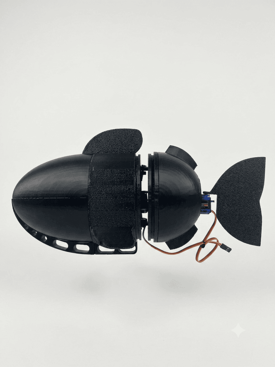
We printed every opaque structural part in black PETG, which hides FDM layer lines, while the nose dome was sourced separately as a transparent part so it could double as a camera window. The full assembly came off five build plates, consuming 473 g of filament over roughly 32 hours and 25 minutes.
Post-processing turned printed parts into a watertight vehicle: supports clipped off, surfaces dressed from 120 up to 240 grit, mating flanges lapped flat for O-ring sealing, dimensions checked to within ±0.3 mm of CAD, then epoxy-bonded flanges and seated silicone O-rings at the dome. Not everything went smoothly. The big front plate suffered a mid-print delamination when air-conditioning draughts swung the ambient temperature; moving the printer away from the vents fixed it on the reprint. Across all five plates, black PETG proved itself.
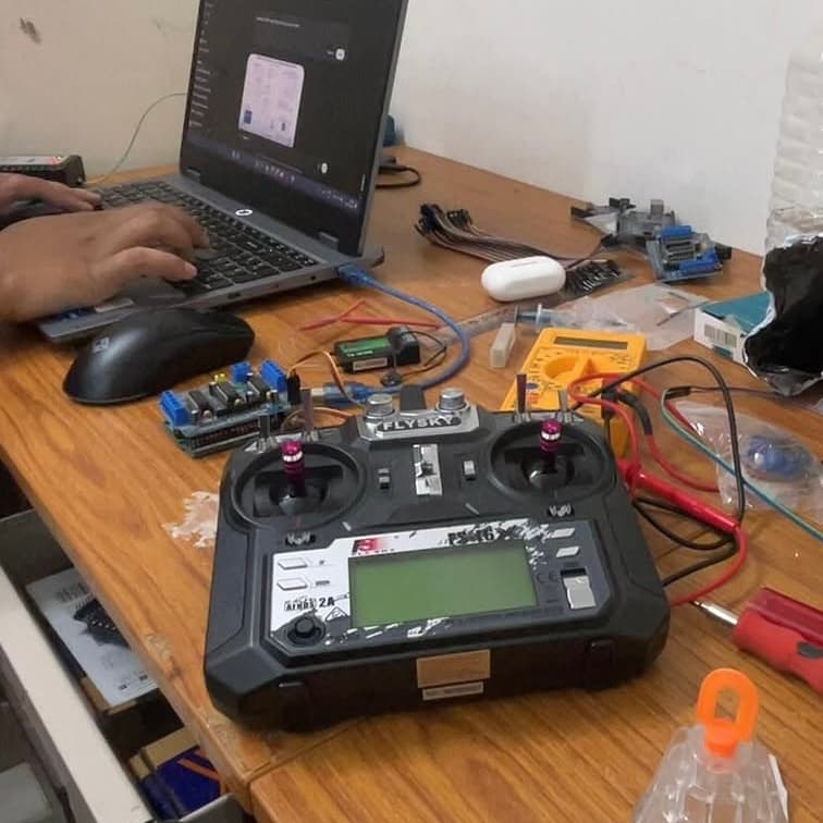
07Wiring its brain
If the hull is the body, the electronics are the nervous system. At the centre sits a microcontroller, an Arduino Nano or a Raspberry Pi Pico, running the control logic and generating the oscillatory signals that drive the motors in a rhythm mimicking natural tail beats. Tune the timing and amplitude of those signals and the robot can swim straight, turn, or spin in place.
Microcontrollers cannot push motor current directly, so a motor driver (an L298N or L9110S) sits in between, amplifying the low-power control signals and shielding the controller from voltage spikes. Two servos do the mechanical work: a small SG90-class servo for steering and a stronger MG90S for the tail. Power comes from a lightweight pack, Li-ion at 7.4 V or Li-Po at 11.1 V, chosen for energy density without weighing the robot down. And because all of this lives underwater, waterproofing is non-negotiable: heat-shrink tubing and silicone sealant protect every exposed connection against shorts and leaks.
08Where the fish learns to swim itself
The near-term roadmap is clear: fold the validated depth model into the full 3D simulation, add real sensors and closed-loop feedback on the physical robot, and push toward autonomous navigation. The more interesting horizon is what happens when the fish stops following hand-tuned rules and starts learning them. Every stage we built turns out to be a foothold for machine learning, and not by accident.
The swimmer is already a gym
Our Simscape model plus the CFD-derived thrust is, almost by accident, a reinforcement-learning environment. Hand-tuned sine waves and three controllers were the baseline; an agent could discover gaits we would never think to try, optimising for cost of transport (distance per joule) instead of raw tracking error. The action is the joint trajectory, the reward is how far it gets on how little battery, and the whole thing trains in simulation before it ever touches water.
A neural stand-in for the CFD
The amplitude sweep was expensive: every angle was a full transient solve. Train a surrogate model on those runs and you get thrust and drag predicted in microseconds across amplitude, frequency, and angle, including where the stall threshold bites. That turns a week of cluster time into a function the controller can call mid-swim, re-optimising its gait online as the water, the payload, or the battery state changes.
Eyes through the dome
We built the nose as an optical window for a reason. A lightweight vision model running on a Pi-class board could turn it into eyes: obstacle avoidance, pipeline following, and learned image enhancement for the turbid, badly-lit water where inspection robots actually earn their keep. The compact size already makes the fish a credible candidate for confined spaces that larger vehicles cannot reach; onboard perception is what would make it autonomous there.
Handing off the controller that fought us
And the depth controller from Stage 5, the one that walked us through four failure modes, is the perfect thing to hand to a learned policy. The time-varying mass and the nonlinear drag are exactly the conditions a model-based RL or MPC controller handles more gracefully than a hand-tuned PID, and it would get there without a human rediscovering integral windup and limit cycles by trial and error.
The big lesson of the whole project is that simplicity is a feature, not a compromise. A two-motor fish cannot do everything a soft-bodied research platform can, but it is cheap to build, honest to reason about, and a genuinely good teaching tool. It is also, it turns out, the perfect substrate to learn on: every honest model we built to understand the fish is a model an agent can now train inside.
Every honest model we built to understand the fish is a model a machine can now learn to swim inside.
What comes next
For now, we have a robot fish that swims. And that started, as these things do, with a sketch in SolidWorks and a question about how fish actually move.
Built by Dameshua Steven Warjri and Gaurav Joshi, Department of Mechanical Engineering, NIT Meghalaya, under the supervision of Dr. Bikash Kumar Sarkar and Dr. Subhendu Maity.

I build scalable products from the ground up: ticketing infrastructure, government platforms, and the backend systems that hold them together under load. Occasionally I help build a robot fish. I write up the ones with interesting failure modes.